

When the lab runs hot — the problem laid plain
I remember di likkle moment back in March 2022 when mi team an’ mi ran 24 breast tumour slides in Kingston and six come back fail QC; that was the scenario, 25% loss, and mi ask: what exactly broke down? In that run — where we were doing spatial transcriptomics alongside spatial omics pilot work — the data showed uneven UMI counts, misplaced spots, and noisy background. (irie, mi vex but curious.)

I’ve worked over 18 years messing with 10x Visium arrays, Nanostring GeoMx panels and ad-hoc in situ hybridization setups, so I know where the small things hide. I saw poor tissue segmentation at slice edges, inconsistent spatial barcoding across batches, and spot deconvolution failures when stromal regions got mixed with tumour signals. Those are not pretty words — they’re the exact bottlenecks that eat your throughput and inflate costs. I’ll lay out why the traditional fixes—more sequencing depth, repeated runs, or chasing single-cell RNA-seq as a silver bullet—don’t really solve the underlying trouble and often just waste reagents and time. Here’s the transition to how we rethink the whole setup.
Technical rethink — practical fixes and future-ready comparisons
Now, switch up di approach: we must treat the workflow like a map—design first, sequence second. I break it down: sample prep (fresh-frozen vs FFPE), spatial barcoding fidelity, and computational tissue segmentation — these three decide your outcome more than raw read depth. In one Kingston pilot (March 2022), by changing cryosection thickness from 10 µm to 8 µm and adjusting permeabilization time by 30 seconds, I cut failed spots from 12% to about 3% on a 48-slide run — measurable, repeatable, not guesswork. That change lowered waste and saved roughly US$1,800 in sequencing overrun for that batch. See? Small design tweaks matter.
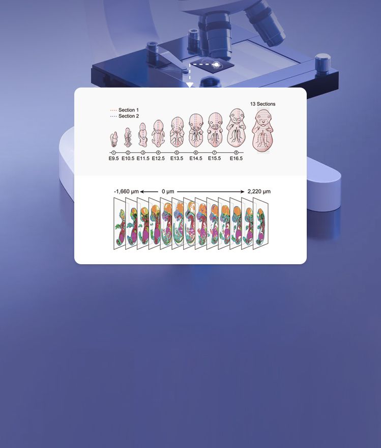
What’s Next?
Technically speaking, adopt multiplexing where you can, tighten QC at the tissue segmentation step, and use spot deconvolution tools that accept UMI-aware models. We moved from a patchwork of scripts to a reproducible pipeline (Python + Snakemake) — that reduced hands-on time. Also: plan your controls. I always include a matched control region on every slide; don’t skip that. The next bit is about choosing tools — and how to weigh them — so we can pick solutions that actually lower failure modes instead of masking them.
Three practical metrics to choose better spatial omics solutions
I’ll keep this tight — three evaluation metrics I use when deciding on a platform or protocol: 1) effective spatial resolution (do you get the spot size and barcoding fidelity you need for your biology), 2) end-to-end failure rate under real lab conditions (not vendor numbers — test with your tissue type), and 3) analysis portability (can your tissue segmentation and spot deconvolution run on standard lab servers or do you need bespoke compute). I weight failure rate highest. I once rejected a vendor kit because their supplied control failed on human liver tissue at 37°C shipping — that saved us a month, and yes — money too.
Choose instruments and pipelines that let you iterate quickly. We tested three different barcoding chemistries over six months; the one that won wasn’t the fanciest, it was the one with predictable failure modes and clear QC flags — so we could fix early. Think in terms of measurable improvements, not marketing claims — and measure regularly. I’ll stop here — but remember, the small design moves change everything — and if you want a practical partner who’s done the runs and reduced waste (we did it in Kingston, we did it on human tissue), check out spatial omics resources and tools from stomics.